When training machine learning models, and deep networks in particular, we typically use gradient-based methods. But if we require the weights to satisfy some constraints, things quickly get more complicated.
Some of the most popular strategies for handling constraints, while seemingly very different at first sight, are deeply connected. In this post, we will explore these connections and demonstrate them in PyTorch.
In particular, we show that mirror descent is equivalent to gradient descent on a reparametrized objective with straight-through gradients: replacing a constrained variable \(x\) with some squishing function \(\sigma(u)\), but treating \(\sigma\) as if it were the identity in the backward pass.
Outline.
Why are constraints challenging?
In machine learning, we fit models to data by minimizing an objective,
Here, \(x\) denotes the parameters to be learned, for instance, the neural network weights. They typically take values in \(\mathcal{X}=\reals\), and we train networks by some variant of the gradient method: we choose an initial configuration \(x^{(0)}\) and successively applying updates of the form:
In deep learning, we typically use stochastic flavors that nonetheless perform well and are efficient. Here, we will focus on a relatively nice example: a convex quadratic function \(f\). We will see that, even in this case, constraints quickly complicate things.
Why constrain? For modeling reasons, we might want to impose restrictions on some of the weights \(x\). Perhaps one of the parameter corresponds to the variance of a distribution, so it cannot be negative. Or perhaps a parameter denotes some sort of “gate”, or mixture between two alternatives \(xa_1 + (1-x)a_2\). In this case, we would need to constrain \(x \in [0, 1]\). This is often called a box constraint and it is one of the most friendly types of inequality constraint we might deal with.
For one-dimensional convex problems, i.e., \(\mathcal{X} = [a, b] \subset \reals\), box constraints do not complicate the problem: we can solve the unconstrained problem \(x_{\text{unc}}^* = \argmin_{x\in\reals} f(x)\). If the answer satisfies the constraint, then it must be the solution of the constrained problem as well. If not, the answer can be found by clipping to the interval:
Proof
We add non-negative dual variables \(\mu_a\) and \(\mu_b\) to handle the inequality constraints \(x \geq a\) and \(x \leq b\), and write the Lagrangian,
An optimal \(x^\star\) must satisfiy the original constraints \((a \leq x^\star \leq b)\) and be a stationary point of the Lagrangian:
The dual variables must be non-negative and satisfy complementary slackness:
Let \(x^\star_\text{unc}\) be the solution of the unconstrained problem, satisfying \(f'(x^\star_\text{unc})=0\). If \(a \leq x^\star_\text{unc} \leq b\), then \(x^\star=x^\star_\text{unc}\), and choosing \(\mu_a=\mu_b=0\) satisfies all conditions.
Otherwise, \(x^\star_\text{unc}\) is either too small or too large. Assume \(x^\star_\text{unc} > a\) and take \(x^\star = a\). Then we have \(\mu_b=0\), and from (F) we must have \(\mu_a = f'(a)\). Is this a valid value for the dual variable? We must check that \(f'(a) \geq 0\). Convex \(f\) satisfies \( f(a) - f(x) \leq f'(a)(a-x) \) for any \(x\), including the minimizer \(x=x^\star_\text{unc}\). By assumption, \(a-x^\star_\text{unc} > 0\), so we may divide by it yielding
The case \( x^\star_\text{unc} > b \) follows similarly.
The following interactive demo might convince you that this is true. We show the 1-d function \(f(x) = (x - x_0)^2 / 2\) and its minimizer constrained to \([0, 1]\). Drag the slider to change the location of the unconstrained minimizer \(x_0\).
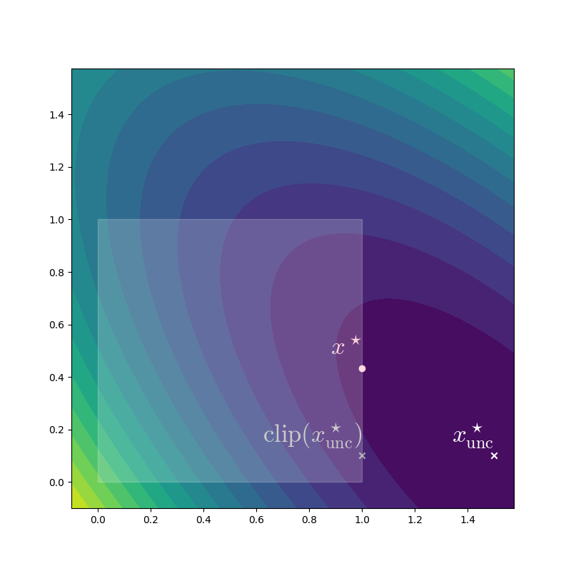
However, in dimension two or more, clipping no longer works, because of interactions between the variables. We demonstate this on a quadratic problem which will become the main focus of the rest of this post,
Let us visualize this problem for the specific case of the unit square \(\mathcal{X} = [0,1] \times [0,1] \subset \reals^2\), with \(x_0 = (1.5, .1)\), and \(Q = \left(\begin{smallmatrix}3 & 2 \\\\ 2 & 3 \end{smallmatrix}\right)\). If not for the constraints, since \(Q\) is positive definite, the minimum would be \(x^\star_\text{unc} = x_0\).Because \(f(x_0)=0,\) and positive definiteness guarantess \(f(x) > 0\) for any \(x \neq x_0\). But a contour plot shows that the constrained minimum \(x^\star\) is not the same as the result of clipping the unconstrained minimum to the box.
Constraint handling cannot be left as an afterthought: it needs to be baked into the optimization strategy. There is an important special case where (QP) can be solved exactly: the case \(Q = I\). In this case, the problem becomes \(\argmin_{x \in \mathcal{X}} \| x - x_0 \|^2_2,\) which is known as the Euclidean projection of \(x_0\) onto \(\mathcal{X}\). If \(\mathcal{X}\) are box constraints, the projection decomposes into a series of independent 1-d projections, which we’ve seen can be solved by clipping.
As a warm up, let us implement our quadratic function \(f(x) = \frac{1}{2} {(x - x_0)^\top}Q{(x - x_0)}\) in PyTorch, as well as a minimal gradient descent loop from scratch.
import torch

torch.set_default_dtype(torch.double)

x0 = torch.tensor([1.5, .1])
Q = torch.tensor([[3.0, 2.0],
                  [2.0, 3.0]])

def f(x):
    z = x - x0
    Qz = z @ Q
    return 0.5 * torch.sum(z * Qz, dim=1)


def optim_grad(x_init, lr=.1, max_iter=100):
    x = x_init.clone().requires_grad_()

    for i in range(max_iter):
        f(x).backward()
        x.data -= lr * x.grad
        x.grad.zero_()

    return x
This procedure quickly converges to \(x^\star_\text{unc} = (1.5, .1)\).
Ways to deal with constraints.
When faced with a box-constrained optimization problem, these are the ideas that most practitioners would turn to.This turns out to be a handy personality quiz to see if somebody resonates more with neural networks or with convex optimization.
-
Reparamtrization (REP). Circumvent the constraints on \(x\), by expressing the function in terms of unconstrained variables \(u\) such that \(x_i = \sigma(u_i)\), where \(\sigma : \reals \to \mathcal{X}\) is a “squishing” nonlinearity. We can then perform unconstrained minimiziation on \(f \circ \sigma\). For \(\mathcal{X}=[0,1]^d\), we may use the logistic function,General intervals \([a,b]\) are obtained by affinely transforming \([0,1]\).
\[ \sigma(u) = \frac{1}{1 + \exp(-u)}\,.\] -
Projected gradient (PG). Perform unconstrained gradient updates, then project back onto the domain after each update:
\[ \begin{aligned} x^{(t+½)} &\leftarrow x^{(t)} - \alpha^{(t)} \nabla f(x^{(t)})\,, \\ x^{(t+1)} &\leftarrow \operatorname{Proj}_\mathcal{X}\big(x^{(t+½)}\big)\,. \\ \end{aligned} \]
REP is convenient when working with neural network libraries like PyTorch, because it can be implemented just by changing our model, without requiring modifications to the optimization code. However, the resulting problem (after reparametrization) is no longer convex in \(u\), even if the original problem was convex in \(x\). PG directly solves the convex optimization problem (QP), but the intermediate iterates \(x^{(t+0.5)}\) can leave \(\mathcal{X}\), leading to a possibly less stable or too aggressive trajectory.
In this post, we will explore the connection between the two by studying mirror descent and its information-geometric interpretation as natural gradient in a dual space. But first, let’s explore our two initial ideas.
Reparametrization.
Instead of optimizing w.r.t. the constrained variables \(x\), we introduce an underlying variable \(u\), such that \(x_i = \sigma(u_i)\).This seems to be the more common method among neural network practitioners; one place where it shows up often is neural variational inference, where we would constrain the variance of a learned distribution using a softplus function. In our case, we use a logistic sigmoid reparametrization to get the unconstrained non-convex problem
where \(\sigma\) is applied element-wise.
When reparametrizing, \(x\) is no longer a learned parameter, but a function of
the learned parameter \(u\). The gradient with respect to \(u\) can be handled
automatically by PyTorch autodiff:
def optim_reparam(u_init, lr=.1, max_iter=100):
    u = u_init.clone().requires_grad_()

    for i in range(max_iter):
        f(torch.sigmoid(u)).backward()  # compute grad wrt u
        u.data -= lr * u.grad  # take gradient step
        u.grad.zero_()

    return u
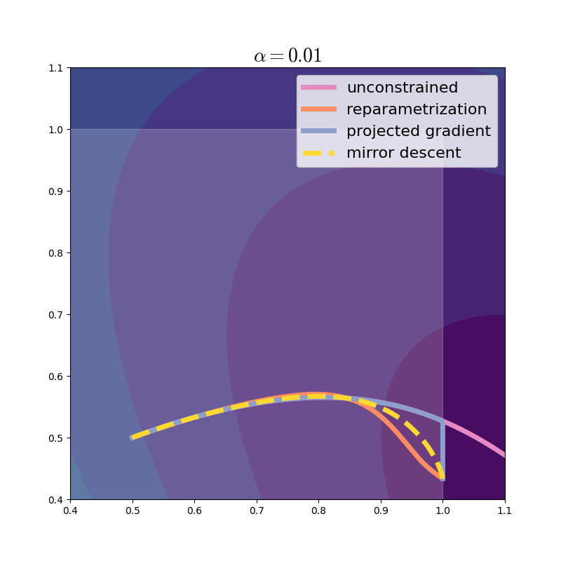
With a very small learning rate, we get a glimpse into the dynamics of this method.As the learning rate goes to zero, we are simulating a continuous gradient flow, of which gradient descent is a discretized approximation. For more about gradient flows, check out Francis Bach’s post. For comparison, we include the unconstrained trajectory.

In practice, we would use a much larger learning rate to accelerate optimization:
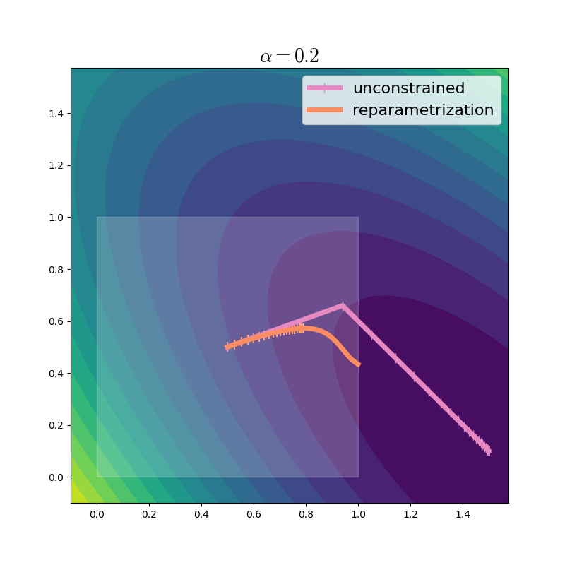
We can see that even with a large learning rate, the reparametrization method takes much smaller steps, especially as it gets closer to the boundary of the domain. The steps are so small, that we only show the first 20 markers, to avoid clutter. Why does this happen? At any point \(u\), the reparametrized gradient can be written using the chain rule:
This is the unconstrained gradient at \(x=\sigma(u)\), rescaled by the Jacobian of \(\sigma\). Since \(\sigma\) acts elementwise, its Jacobian is a diagonal matrix, with \(\pfrac{\sigma(u)_i}{u_i} = \sigma(u_i)(1 - \sigma(u_i)) = x_i (1 - x_i).\) We can thus see that as \(x_i\) approaches \(0\) or \(1\), the reparametrization rescales the gradient severely, bringing the effective step size toward 0. It can help to see the concrete values and shapes of these matrices:
Calculation
Let’s consider two points: first far, then close to the optimum. We use that \(\nabla_x f(x) = Q(x - x_0)\). (Note: all vectors below are column vectors.)
| \(u\) | \({x=\sigma(u)}\) | \(\pfrac{\sigma(u)}{u}\) | \(\pfrac{f(x)}{x}\) | \(\pfrac{f(\sigma(u))}{u}\) |
|---|---|---|---|---|
| \((0, 0)\) |
\((.5, .5)\) | \(\left(\begin{smallmatrix} .25 & 0 \\\\ 0 & .25 \end{smallmatrix}\right)\) | \((-2.2, -0.8)\) | \((-0.55, -0.2)\) |
| \((4.6, -0.4)\) | \((.99, .4)\) | \(\left(\begin{smallmatrix} .0099 & 0 \\\\ 0 & .24 \end{smallmatrix}\right)\) | \((-0.93, -0.12)\) | \((-0.01, -0.03)\) |
Two effects are at play here: the gradient of \(f\) gets smaller as we approach the minimum, and the gradient of \(\sigma\) gets vanishingly small as we approach the boundary of the domain.
Remember, this rescaling happens automatically through the chain rule! But, although slowly, and along a slightly winding trajectory, our method finds the right answer.
Projected gradient.
The projected gradient method is particularly well suited to handling “simple” constraints like the box case, but, unlike reparametrization, requires a different kind of expertise to get running in the case of complicated constraints.PG is very popular in convex optimization, useful both for theory and for practice. However, it does not seem to be so widely used in the pure neural network world, perhaps mostly because it is not directly supported by the built-in optimizers in major frameworks. For box constraints, the projection can be computed efficiently, since \(\big[\!\operatorname{Proj}_{[0,1]^d}(x)\big]_i = \operatorname{clip}_{[0,1]}(x_i).\) The implementation follows:
def optim_pg(x_init, lr=.1, max_iter=100):
    x = x_init.clone().requires_grad_()

    for i in range(max_iter):
        f(x).backward()
        x.data -= lr * x.grad  # take gradient step
        x.data = torch.clamp(x.data, min=0, max=1)  # project
        x.grad.zero_()

    return x
Let’s visualize the trajectory. From now on, we will zoom in a bit on the region of interest.
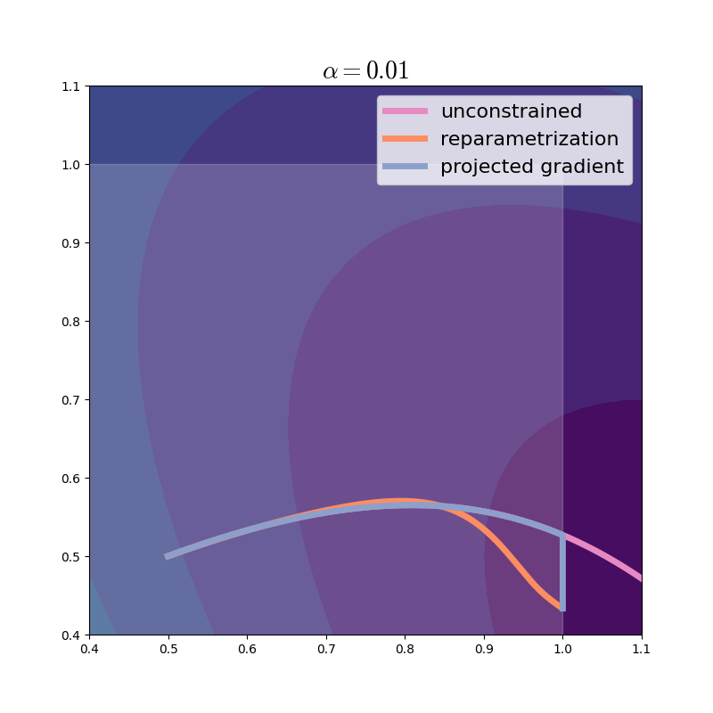
It looks like the projected gradient method tends to follow the unconstrained trajectory while sticking to the boundary of the domain. Of course, with larger steps, the differences become more pronounced.
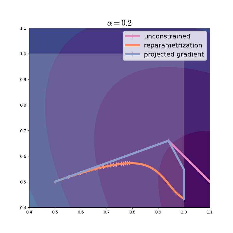
In this instance, PG is the clear winner: look how fast it makes progress. With less well-behaved and non-convex functions this need not be the case. So we are motivated to delve deeper and explore how PG and REP relate, despite seeming so different.
Generalizing the projected gradient method with divergences.
In the projected gradient method, we take unconstrained steps, which might take us outside of \(\mathcal{X}\), and then move the solution back to \(\mathcal{X}\) by projection:
Projection finds the point \(x \in \mathcal{X}\) closest to \(x^{(t+½)}\), i.e.,
The projected gradient update can be interpreted as minimizing a regularized linearization of \(f\) around the current iterate,
Explanation
Why does this update make sense, and where does it come from? We are trying to minimize a function \(f(x)\), but we don’t know what it looks like globally: we only have access to its value \(f(x)\) and its gradient \(\nabla f(x)\) at points \(x\) that we may query one at a time. At any point \(x_0\), the first-order Taylor expansion is:
To get a linear approximation of \(f\) we can plug in \(\delta = x - x_0\):
So as long as \(x\) is not too far from \(x_0\), we have
This affine approximation is much easier to minimize, but it is only accurate locally, therefore, we use it iteratively, taking a small step, then updating the approximation:
where the term on the right keeps us close to \(x^{(t)}\) to ensure the approximation is not too bad. Clearing up the constant terms from inside the \(\argmin\) yields the desired expression.
Rearranging the terms reveals exactly the projected gradient update,
Derivation
Now, let’s pay special attention to the function \(D(x, y) = \| x - y \|^2 = \sum_i (x_i - y_i)^2\), the squared Euclidean distance. We employ this function to ensure that each update stays close to \(x^{(t)}\), because the linear approximation is not good if we go to far. But this is not the only good measure of closeness: here, geometry enters the stage! Euclidean geometry is convenient and comfortable for thinking about spaces like \(\reals^d,\) but it is not always the best model.
Bregman divergences provide a convenient generalization of the squared Euclidean distance: Divergences measures of dissimilarity between objects, with weaker requirements than distance functions: simply that \(D(x,y) \geq 0\) and \(D(x,y)=0\) iff. \(x = y\). Bregman divergences are an important class of divergences. They are convex in the first argument, but not the second. given strictly convex, twice-differentiable \(\Psi\),
For \(\Psi = \frac{1}{2} \| \cdot \|^2\), this recovers the squared Euclidean
distance. Replacing \(\frac{1}{2}\|\cdot\|^2\) by \(D_\Psi\) in the projected
gradient algorithm leads to a generalization known as mirror descent,
Introduced in:
A.S. Nemirovsky and D.B. Yudin,, 1983. Problem complexity and method efficiency in optimization.
Suggested reading:
A. Beck and M. Teboulle, 2003.
Mirror descent and nonlinear projected subgradient methods for convex optimization.
Operations Research Letters, 31(3). 167-175.
Since \(\Psi\) is twice differentiable and strongly convex, it has a gradient \(\psi = \nabla\Psi\) which is invertible. Solving for the mirror descent update yields a so-called Bregman projection, or non-linear projection,
If \(\Psi\) is carefully chosen such that \(\psi^{-1}(u) \in \mathcal{X}\) for all \(u \in \mathcal{U}\), then the Bregman projection step is trivial, yielding
Let’s make this more concrete.
The choice of \(\Psi\) will define the geometry of our space. Values in \([0,1]\) may be interpreted as coin flip probabilities: the higher, the more likely an event is to happen. An important property of a binary random variable is its entropy. If \(x_i \in [0, 1]\) denotes the probability associated with coin \(i\), the entropy is
We may extend this additively to vectors as \(H(x) = \sum_i H(x_i)\).
This is sometimes called the Fermi-Dirac entropy. On \(\mathcal{X}=[0, 1]\), entropy is continuously differentiable and strictly
concave, maximized at \(x=0.5\) and minimized at \(x=0\) and \(x=1\).\(H(0.5) =
\log 2,\)
\(H(0)=H(1)=0\).
Let us thus take \(\Psi = -H\). Its gradient is \(\psi : \mathcal{X} \rightarrow \mathcal{U}\),
with inverse \(\phi : \mathcal{U} \rightarrow \mathcal{X}\),
So, written in terms of the familiar logistic sigmoid, the mirror descent update induced by the negative entropy takes the (remarkable!) form
Things are beginning to clear up! We can think of the pair of inverse functions \((\psi, \phi)\) as maps between \(\mathcal{X}\) and \(\mathcal{U}\). We will call these the primal and dual spaces, respectively.Duality, and the terms primal and dual, are fairly strong, scary, and sometimes overloaded. Readers familiar with the Fenchel conjugate, \(\Psi^*(u) \coloneqq {\sup_{x} \{ \DP{u}{x} - \Psi(x) \},}\) should note note that \(\Psi^* = \Phi\), where \(\Phi\) is such that \(\nabla\Phi = \phi\). (For the Fermi-Dirac entropy, \(\Phi(u) = {\log(1+\exp(u)).}\)) The dual construction used here relies on the relationship between Bregman divergences and Fenchel conjugates: \( D_{\Phi^*}(u, v) = D_\Phi(y, x)\) where \(u=\psi(x), v=\psi(y)\) are the dual points corresponding to \(x\) and \(y\). Mirror descent thus first moves into dual (unconstrained) space, performs an update there, and then moves back. Reparametrization rewrites the problem in dual coordinates and performs gradient descent: this is not the same, and the trajectories are quite different!
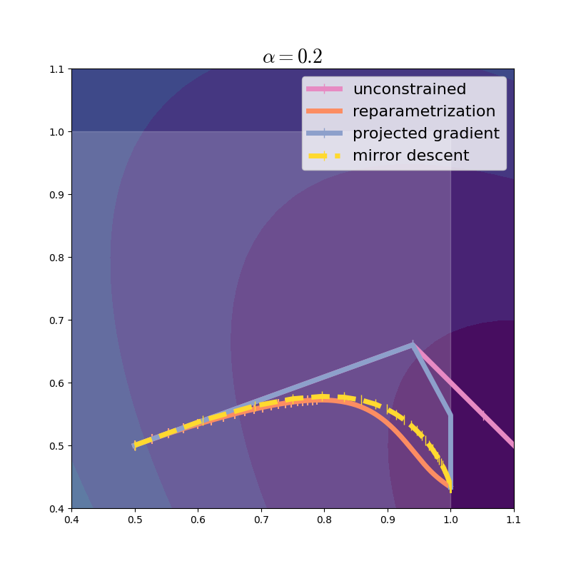
With a larger step size, we see that mirror descent takes much larger steps than reparametrization does.
Now that we figured out that we may think about the problem in primal or dual coordinates, we may also visualize the optimization trajectory in dual coordinates.
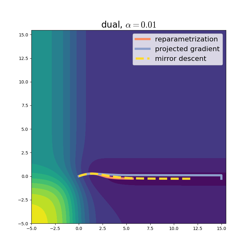
Yet, the way that mirror descent leans on moving from \(\mathcal{X}\) to \(\mathcal{U}\) is very familiar to the reparametrization strategy. Is there a deeper connection between the two? We illuminate it next.
Duality between mirror descent and natural gradient.
We have seen that different choices of \(\Psi\) induce different geometries even on top of the same space. (Case in point: entropy vs. \(\frac{1}{2}\|\cdot\|^2\)). To handle this ambiguity, we need a structure that attaches the geometry along with the underlying space. This, (with some handwaving), is a Riemannian manifold: a pair \((\mathcal{U}, G)\) where \(\mathcal{U} \subseteq \reals^d\) is an underlying spaceRiemannian manifolds are more general than this, but in this post, for simplicity, we only look at the case where \(\mathcal{U}\subseteq \reals^d\). To be fully general, the notation ramps up quickly. See Agustinus Kristiadi’s post and Frank Nielsen’s tutorial for an introduction. and \(G: \mathcal{U} \rightarrow \reals^{d \times d},\) known as the metric tensor, is a function that takes a point \(u_0\) on the manifold and returns a positive definite matrix that characterizes the geometry by specifying a custom squared distance nearby \(u_0\):
What we observed earlier is in fact a duality between the Riemannian manifolds \((\mathcal{X}, \nabla^2 \Psi)\) and \((\mathcal{U}, \nabla^2 \Phi),\) where \(\Phi\) is the antiderivative of \(\phi\), i.e., \(\nabla\Phi=\phi\). This is an important duality studied in the field of information geometry. S. Amari, A. Cichocki. 2010. Information geometry of divergence functions. Bulletin of the Polish Academy of Sciences, 58(1).
We may now revisit the reparametrization strategy, in light of what we learned so far. To reparametrize the constraint away, we work in dual coordinates \(u \in \mathcal{U}\), and update:
In our case \(\mathcal{U}=\reals^2\) and \(\phi = \sigma\), but let’s use the more
general notation. The update above ignores the geometry of \(\mathcal{U}\), in
other words, operates on the trivial manifold \((\mathcal{U}, I_d)\) — the
metric tensor is the identity matrix everywhere. When optimizing some function \(\tilde{f}(u)\)
over a Riemannian manifold \((\mathcal{U}, G)\),
a convenient algorithm is natural gradient,S. Amari, 1998.
Natural gradient works efficiently in learning.
Neural computation 10.2, 251-276.
which takes the form
Derivation
We follow the same steps as for gradient descent, but we use the induced distance \(d_{u^{(t)}}\) to find an update direction. We must solve the problem
Rearranging gives the equivalent problem
Assuming no constraints (i.e., \(\mathcal{U}=\reals^d\)), this yields the desired update.
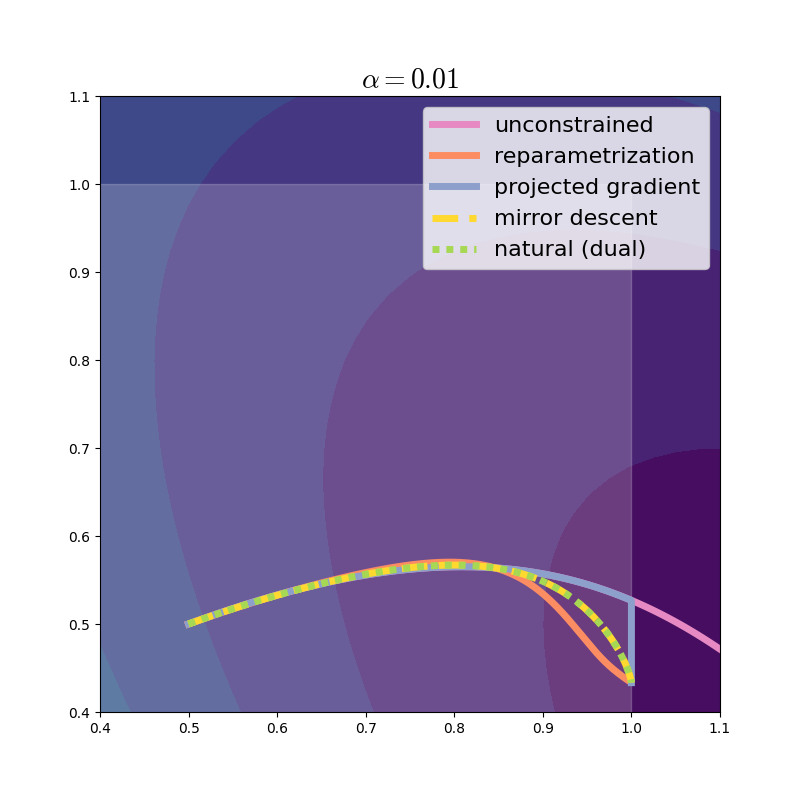
It turns out that for a pair of Bregman dual manifolds \((\mathcal{X}, \nabla^2 \Psi)\) and \((\mathcal{U}, \nabla^2 \Phi),\) mirror descent in the primal space is equivalent to natural gradient in the dual space! This result, due to Raskutti and Mukherjee (2015), G. Raskutti and S. Mukherjee. 2015. The information geometry of mirror descent. In: IEEE Transactions on Information Theory, vol. 61, issue 3. arXiv:1310.7780. means we can get a geometry-aware flavor of the REP algorithm,
This algorithm produces the exact same iterates as mirror descent, but — since it maintains iterates in dual space — is more numerically stable. A first attempt at implementing natural gradient is:
def optim_rep_natural(u_init, lr=.1, max_iter=100):

    u = u_init.clone().requires_grad_()

    for i in range(max_iter):
        x = torch.sigmoid(u)
        dsigmoid = (x * (1 - x)).detach()  # diagonal of ∇²Φ(u)
        f(x).backward()
        u.data -= lr * u.grad / dsigmoid
        u.grad.zero_()

    return u
and we can visually check that we get exactly the same trajectory as mirror descent.
But let’s look a bit closer! Since \(\phi = \nabla\Phi\), our metric tensor is none other than
and, putting the whole update together, we see that
Natural gradient cancels out the Jacobian of \(\phi\) in the chain rule!
This suggests an alternative implementation,
reminiscent of straight-through tricks: we use a reparametrization function
\(\sigma\) that is a sigmoid in the forward pass, but acts as if it were the
identity in the backward pass.
Such “straight-through” heuristics are very popular for dealing with
stochastic or piecewise-constant functions (like argmax or floor functions.)
To my knowledge, the idea was introduced by G. Hinton in the Neural Networks for
Machine Learning online lectures in 2012. For a detailed treatment, see:
Y. Bengio, N. Léonard, A Courville. 2013.
Estimating or Propagating Gradients Through Stochastic Neurons for Conditional Computation.
arXiv:1308.3432.
class SigmoidStraightThrough(torch.autograd.Function):

    @staticmethod
    def forward(ctx, u):
        return torch.sigmoid(u)

    @staticmethod
    def backward(ctx, dx):
        return dx


def sigmoid_straight_through(u):
    return SigmoidStraightThrough.apply(u)


def optim_rep_natural_st(u_init, lr=.1, max_iter=100):

    u = u_init.clone().requires_grad_()

    for i in range(max_iter):
        f(sigmoid_straight_through(u)).backward()
        u.data -= lr * u.grad
        u.grad.zero_()

        print(u.data, torch.sigmoid(u.data))

    return u
With this sigmoid_straight_through nonlinearity, we can now use mirror descent
/ natural gradient to learn constrained parameters without any changes to the
optimizer, and with improved numerical stability.Instead of cancelling out
the gradient of \(\sigma\) numerically, we now avoid multiplying by it in the
first place. Unlike our initial reparametrization algorithm, this algorithm uses the
geometry of the dual space \((\mathcal{U}, \nabla^2\Phi)\) and thus avoids taking
extra small steps while still ensuring that all the iterates remain feasible.
Conclusions.
We have explored the two most popular strategies for dealing with simple constraints: reparametrization and projected gradient optimization. We have looked into an information geometric generalization of projected gradient, which turns out to lead to an equivalent dual algorithm that resembles reparametrization, but with a gradient correction that improves its performance. (And, if \(f\) is convex, results in a convex optimization procedure, unlike the reparametrized case.)
Of course, we only looked at a simple quadratic test case, and we did not check what happens when using accelerated methods or adaptive learning rates (e.g,. Adam). But empirical questions are not the main point.
With this post, I have hopefully stirred your interest into constrained optimization and its connections to geometry. You may be wondering what other constraints we may handle this way. Two important examples are non-negativity constraints \(\mathcal{X}=[0, \infty)^d,\) for which we may use \(\Psi(x) = \sum_i x_i(\log x_i - 1),\) giving \(\phi(u) = \exp(u)\),Another interesting choice is \(\Psi(x) = x \log(\exp(x)-1) + \operatorname{Li}_2(1-\exp(x)),\) where \(\operatorname{Li}_2\) denotes the dilogarithm. This leads to the softplus reparametrization \(\phi(u) = \log(1+\exp(u))\). While the dilogarithm lacks a closed-form expression, we only need to evaluate \(\phi\) and \(\psi\). and the simplex \(\mathcal{X} = {\{ x \in \reals^d : x_i \geq 0, \sum_i x_i = 1 \},}\) for which the negative Shannon entropy \(\Psi(x) = {\sum_i x_i \log x_i}\) yields the softmax reparametrization \(\phi(u) = {\frac{1}{Z} \exp(u)}\) with \(Z=\sum_i\exp(u_i).\) The resulting simplex-constrained algorithm is known under many names, including “multiplicative weights”, “entropic descent”, or “exponentiated gradient”. J. Kivinen, J and M.K. Warmuth, 1997. Exponentiated gradient versus gradient descent for linear predictors. Information and Computation, 132(1), 1-63. This algorithm performs the elementwise multiplicative update
More interesting constraint examples involve matrices. Geometric insights have been key to advances in learning over constrained spaces of matrices, such as symmetric, low-rank, orthonormal, positive (semi-)definite matrices, etc. P.-A. Absil, R. Mahoney, and Rodolphe Sepulchre. 2008. Optimization Algorithms on Matrix Manifolds. Princeton University Press. ISBN 978-0-691-13298-3 Schäfer et al. use the duality between mirror descent and natural gradient to derive powerful algorithms for minimax problems. F. Schäfer, A. Anandkumar, H. Owhadi. 2020. Competitive Mirror Descent. arXiv:2006.10179.
Acknowledgements.
This post was inspired by Anima Anandkumar’s talk at the IAS Seminar on Theoretical Machine Learning. Before this talk, I had no idea about anything in the second part of this post. Thanks to Mathieu Blondel, Caio Corro, André Martins, Fabian Pedregosa, and Justine Zhang for feedback, and to all Twitter users who pointed out typos. I am funded by the European Research Council StG DeepSPIN 758969 and Fundação para a Ciência e Tecnologia contract UIDB/50008/2020.
Comments !